

Effective ground testing is an informed combination of instrumentation and procedure. Accuracy, resolution, safety, noise suppression, graphics, clamp features, and general reliability are all critical, as they are with any electrical testing. But effective and accurate ground testing depends as much on adherence to procedure as it does on quality of instrumentation. If the operator does not understand and diligently apply correct procedure, the highest quality instrument will be little more than a waste of money. Some relatively common electrical tests basically amount to connecting a pair of leads and pressing a test button, but not so ground testing! Random hookup and intuitive operation get the operator nowhere.
Fall of Potential
The basis for ground testing is found in the fundamental procedure known as fall of potential (FOP). A long test lead — often as long as the operator can provide or manage — is stretched out with a metal rod or probe clipped to the end. When the tester is energized, a current circuit is established by an alternating square wave through the soil to the electrode being tested. The unique frequency of the square wave provides a test signal against which the tester can measure.
Measurement is accomplished by means of the second test circuit: potential. A long lead is similarly strung out, and a metal probe is driven into the soil. This is normally in the direction of the current probe but need not be if obstructions impede. This circuit measures voltage drop caused by soil resistance, and the two measured parameters — current and potential — calculate resistance through Ohm’s Law. The tester displays resistance to the location point of the potential probe.
This may sound simple, but it isn’t. The problem lies in determining just what is being measured. Move the potential probe, and the tester will calculate a new resistance to the new location. Even if the distance to the probe is maintained constant but in a different direction, the reading may differ. This is due to local soil anomalies from one probe placement to another. This is where correct procedure defines a reliable test. Indeed, if no study is done by the operator and the leads are merely stretched out for their lengths and a reading taken, a correct measurement may be achieved. Unfortunately, this is often done in the field, but it is pure luck.
The correct procedure is to take an arbitrary number of measurements in a line and graph the distance at which the reading was taken versus resistance at that point (Figure 1).
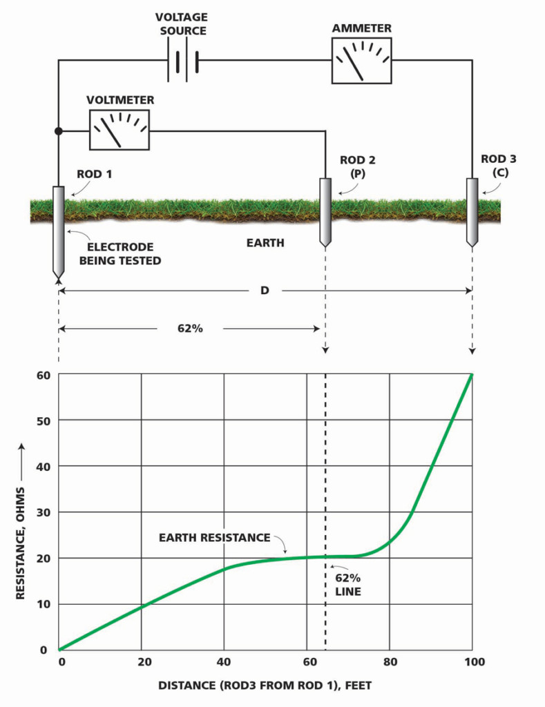
Figure 1: Successful FOP Test with Instrument Setup
What is hoped for is a level graph line at a satisfactorily low value. This accomplishes two things: It identifies the steadily rising graph where the measured ground resistance runs directly into the extraneous resistance of the current probe, and it reveals local soil inconsistencies that could severely distort a single reading (Figure 2).
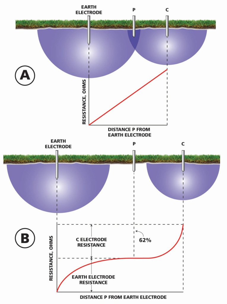
Figure 2: Comparison of Failed and successful FOP Graphs. The continuously rising graph line (top) may include correct resistance reading, but it is unrecognizable. The extended horizontal line in the correct test (bottom) clearly identifies ground resistance.
Simplified Fall of Potential
Fall of potential is the best overall method, but it requires considerable work and possibly too much room to stretch leads. What then? Other methods have been derived, some for the purpose of saving time and others for dealing with difficult test conditions. The first of these, called simplified fall of potential, requires only three measurements rather than enough to draw a graph line for possibly hundreds of feet. A simple and easy mathematical proof substitutes for drawing the graph. The most atypical of the readings is mathematically compared to the average and then calculated as a percentage accuracy. The operator makes a decision as to whether this is an acceptable accuracy. If so, the average is submitted as the test result. If all three readings were the same, then this would provide added assurance. But non-homogeneity of soil, especially around graded construction sites, often precludes this.
An obvious spinoff here is to dispense with any math and merely move the potential probe back and forth a few times and decide whether the readings fall reasonably well together. This could be referred to as the eyeball method. It lacks genuine method but is probably the most widely used procedure, at least for less demanding locations. An experienced operator may indeed have sufficiently keen powers of discernment, but if third parties are involved (i.e. inspectors, clients, insurance, lawyers), it may be more practical to do the math and submit the report.
62% Rule
Finally, the 62% rule brings simplicity down to its base level. Mathematics tracing back to the ancient Greek scholars supports the 62% rule. But none of that is necessary to apply to ground testing. All the ground test operator needs to know is that the 62% position on an FOP graph is the one that will give the most accurate reading.
So why aren’t all ground test readings taken at that position and be done with it? The answer is because the mathematics is based on an ideal model, and few construction sites, industrial sites, or anywhere else are likely to conform to ideality. Grading mixes topsoils from different locations. The soil may be naturally stony. There may be a large subterranean rock, power cable, water main, ground water, or other non-uniformity to contend with. Put simply, the reading at 62% may not be representative. It is accepted at the operator’s risk unless the site has previously been proven by more rigorous prospecting. The rule is a quick and handy backup test on sites where distances and directions have been established by rigorous testing. But a new test runs the risk of a gamble.
Slope
The other reason for established test procedures is to effectively address difficult situations. The main challenge is insufficient space in which to extend test leads far enough to separate the resistance field around the current probe from that of the electrode being measured. A coherent FOP graph cannot be constructed, and the graph line continues to rise as more resistance is added with each move of the potential probe. By far the most popular means of dealing with this issue is the slope method (Figure 3).
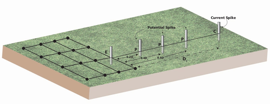
Figure 3: Typical Slope Method Layout
If the graphed resistance line continues to rise, most likely the correct value is there somewhere — it just can’t be discerned from viewing the graph. Still, even a partial FOP graph can come in handy. Only three measurements are necessary for the proof. These are at 20%, 40%, and 60% of the distance to the current probe. From these three numbers, a slope coefficient, typically referenced by the Greek letter μ, is calculated and referenced to a table commonly available in the ground testing literature. As the slope coefficient represents the distance to the potential probe over the distance to the current probe and the latter is known, the distance at which the correct ground resistance reading should be taken is calculated by solving this simple equation: dp/dc = μ for dp.
The actual ground resistance reading can then be determined by either reading the graph line or physically placing a potential probe at that distance and taking the reading. But suppose the calculated μ value cannot be found on the table? That would indicate the resistance field of the current probe is contained completely within that of the test ground and cannot be successfully determined. What then?
Intersecting Curves
The fallback is intersecting curves. This is a difficult and tedious procedure to be avoided if possible, but it works when nothing else will. Two sets of graphs are constructed. One set is of three portions of FOP graphs working from an edge of the grid. These will keep rising. If they did not, they would be complete FOP graphs and intersecting curves wouldn’t be necessary. But since these are not readable FOP graphs, where is the 62% distance? For that, a second set of graphs is constructed by selecting arbitrary points for the electrical center of the grid at a distance x from the connection on the edge of the grid and then locating the 62% accordingly. The arbitrary values of x are plotted against the 62% resistances on each of the curves. These three graph lines will coincide at one point (Figure 4) for the correct distance of x from the true electrical center of the grid to the point of attachment of the test lead(s) at the edge. All other values for x are wrong (not the true electrical center), and so the resistances will scatter, with only the correct resistance being common to all three graphs.
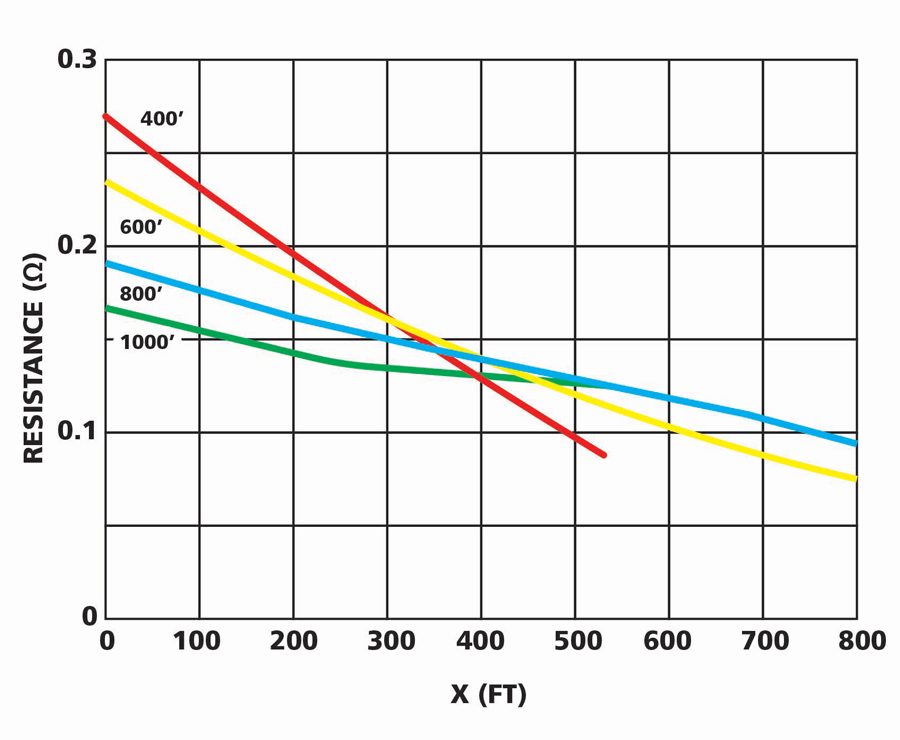
Figure 4: Center of Triangle Formed by Graph Lines is Ground Resistance
Four Potential
Another problem associated with applying FOP to large grids is that their shapes can become more and more asymmetrical, rendering it increasingly difficult to apply even a fair guess as to the electrical center. Since these grids can also have very low resistances, it is easy to fall into incoherent results if a proven method isn’t followed. A means of addressing this is the four potential method, but unlike slope and intersecting curves, it can require prohibitively long leads. The tester is connected to an arbitrary point on the edge of the grid. Leads are stretched in a straight line, and six critical values are taken at 0.2, 0.4, 0.5, 0.6, 0.7, and 0.8 of the distance to the current probe (Figure 5). These results are processed through four simple + and – formulae that yield the correct ground resistance. The four results should substantially agree, imparting confidence to the calculation.
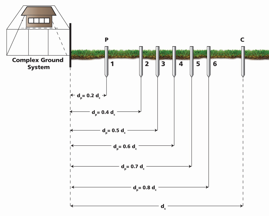
Figure 5: Typical Layout for Four Potential Method
Star Delta
Two methods remain for confines so tight that even minimal extension of current and potential leads is prohibitive. One of these is star delta. The tester is shunted into a two–terminal configuration, either X – PC or C1P1 – P2C2. Modern testers have selector switch positions, and physical shunting is not necessary. Three test probes are placed in a triangle around the ground electrode being tested, and six two-point resistance measurements are taken between each pair of probes and between each probe and the ground under test (Figure 6). Similar to four potential, these six test results are processed through four simple equations for resistance of the test ground, and agreement provides assurance.
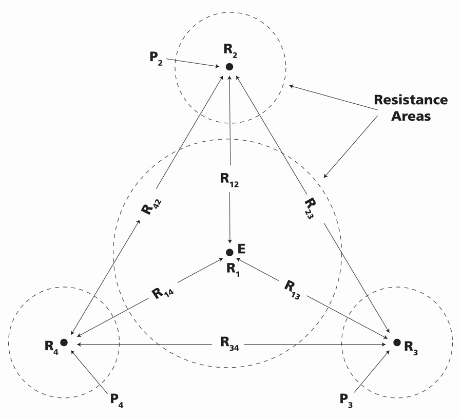
Figure 6: Star Delta Test Configuration
Dead Earth
Finally, under the worst of urban conditions, with virtually no room for leads or place to drive probes, the two-point star delta test becomes the only option. The second test lead is attached to any convenient low-resistance return: a metal fence post, building structure, or best of all, the water pipe system. Test current circulates through the earth to the water pipe system or other connection and back to the tester through a lead (Figure 7). A series loop is measured, and its success counts on the return element being of negligible resistance. This is commonly called the dead earth method because the return is not part of an electrical system. It’s not especially accurate or reliable, but sometimes it’s all that remains.
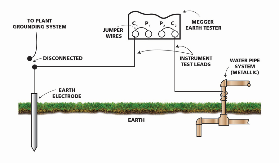
Figure 7: Dead Earth Test Setup
Conclusion
A ground test performed by random hookup will likely yield some result, but it’s no more reliable than rolling dice. Because the earth is so vast, adherence to established procedure is mandatory. Know the procedures, where and why they apply, and results will be trustworthy and effective.
 Jeffrey R. Jowett is a Senior Applications Engineer for Megger in Valley Forge, Pennsylvania, serving the manufacturing lines of Biddle, Megger, and Multi-Amp for electrical test and measurement instrumentation. He holds a BS in biology and chemistry from Ursinus College. He was employed for 22 years with James G. Biddle Co., which became Biddle Instruments and is now Megger.