

Southern California Edison (SCE) began using primary to secondary winding (CHL) narrow band dielectric frequency response (NBDFR) measurements for condition assessment of used distribution class transformers in 2015; 1800 units are evaluated annually. NBDFR is a series of insulation power factor measurements taken from 1–400 hertz, usually at a low voltage. The data derived from the series of CHL measurements constitutes the dielectric response for the transformer. The subsequent evaluation consists of a geometric analysis of the plot where measured power factors and corresponding frequencies are graphed. Insulation condition can be ascertained based on specific characteristics observed within the plot.
Interpretation
Insulation power factor at 60 hertz is the traditional method used to assess the quality of an insulation system. However, because of the magnitude of the capacitive current, a moderate increase in conductive losses will result in a negligible increase in percent power factor at 60 hertz. As the applied frequency is decreased, the effect of capacitive current diminishes while the conductive watt losses remain constant. As a result of this relationship, conductive losses through the insulation become exponentially more visible at lower frequencies. Because of this effect, the narrow band DFR protocol is tremendously sensitive to small changes in insulation condition. This represents a quantum leap in diagnostic reach compared to single-frequency power factor testing.
An ideal response for a typical 15 kV class-95 basic insulation level (BIL) distribution transformer is shown in Figure 1. The portion of the response from 1–10 hertz is dominated by the condition of the oil. The effects of winding geometry are seen in the form of interfacial polarization losses. This accounts for the beginning of the characteristic geometric hump seen at the lower end of the trace indicating deteriorated or contaminated insulation. The portion of the response from 10–100 hertz tends to be dominated by the condition of the cellulose components. The upper end of the response at 400 hertz is mildly influenced by winding geometry as well as the effects of static charge polarization losses.

Figure 1: Characteristics of an Ideal NBDFR Response
With NBDFR, as in conventional testing, the magnitude at 60 hertz will be noted as the condition assessment reference. An earlier interpretation stated that if the slope at 60 hertz was positive at 20°C, then the insulation system in question was deemed to be in acceptable condition. However, this paradigm is an oversimplification, in that the slope at 60 hertz is determined by the location of the point of minimum magnitude or trough. As the insulation and oil deteriorates, the measureable watt losses increase with the generation of polar and conductive contaminates. These losses will distort the low-frequency end of the plot, pushing the entire response (including the trough) toward the upper-frequency end of the plot. In this scenario, the frequency at which the trough resides can be monitored and used as a marker to determine the degree of response migration. While the trough location is very sensitive to an increase in watt losses, the magnitude of a moderate change may not be detectible at 60 hertz.
By establishing a robust database, condition classifications can be established based on trough location. SCE uses this method in combination with magnitude at 60 hertz to determine suitability for refurbishment and reinstallation.
Effects of Aging
When SCE began utilizing the NBDFR protocol in 2015, it became evident almost immediately that, in many cases, trough location migrated very rapidly with very little change in CHL at 60 hertz. To better understand the degradative process as reflected through NBDFR, SCE performed a series of experimental protocols that subjected distribution transformers to prescribed overloads under controlled conditions. The transformers were de-energized on a monthly basis, and NBDFR measurements were performed after units had cooled to ambient temperature. Units that were loaded as per nameplate rating showed minimal changes both in terms of CHL at 60 hertz and trough position. Low-frequency distortion in the responses was also negligible. Conversely, Figure 2 shows the overlaid NBDFR results for a unit operated at 97°C for six months.
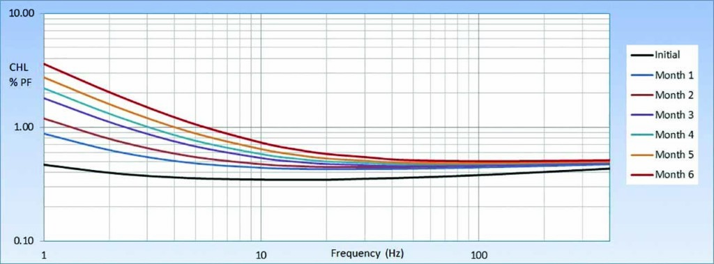
Figure 2: NBDFR Traces for Distribution Transformer Operated at 97°C for Six Months
Examination of the numerical data reveals that the CHL at 60 hertz increased from 0.366% to 0.510% for a difference of 0.144%. Conversely, the CHL at 1 hertz shot up from 0.469% to 3.601% with a difference of 3.132%. While an increase of 0.144% at 60 hertz for a distribution transformer returned from service would be considered normal, the increase at 1 hertz would be alarming. In addition, the trough migrated all the way from an initial position at 15 hertz to 110 hertz after heat cycle #6.
In a subsequent 2017 study, transformers were again subjected to prescribed loads in controlled conditions. Figure 3 shows the NBDFR traces for a unit operated at 120°C. The initial trace is shown in black, with one- and six-month traces depicted in blue and red, respectively. After six months, the magnitude at 1 hertz was measured at 8.146%, which is obviously catastrophic. Proportionally, the trough migrated from an initial location at 20 hertz to a position at 446 hertz. The detail of note in this case is the magnitude at 60 hertz. With the tremendous concentrations of polar compounds in the oil and the contamination of the cellulose components, the assumption should logically be made that the magnitude at 60 hertz would reflect this degradation. However, this is not the case. CHL at 60 hertz actually dropped from 0.530% to 0.487%. In this scenario, the radical movement of the response toward the high-frequency end of the plot results in a situation where the CHL at 60 hertz is no longer a valid parameter. This perfectly illustrates the most significant shortcoming of single-frequency insulation power factor testing.
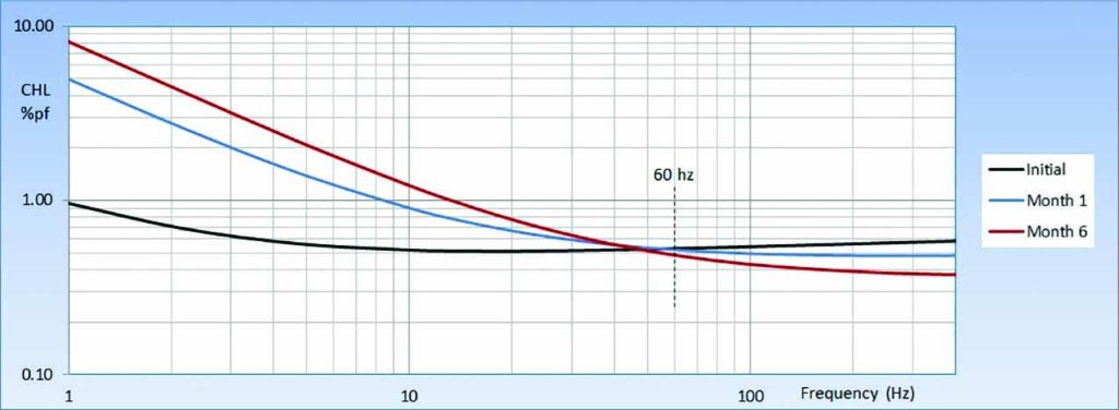
Figure 3: NBDFR Traces for Distribution Transformer Operated at 120°C for Six Months
Bandwidths and Graphic Analysis
Some test equipment utilizes a frequency band ranging from 15–400 hertz. In addition, some equipment uses a linear plot. In Figure 4, the traces from Figure 2 are depicted using the 15–400 hertz linear plot method.
If the linear plot is used in conjunction with the 15–400 hertz measurement, the vital data below 15 hertz seen in Figure 3 is lost. Due to the vertical compression of the trace, trough location cannot be ascertained without consulting the corresponding data table. In this case, most of the traces in Figure 4 still provide evidence of transformer degradation. However, in cases of mild degradation, this method and format will prove problematic. The obvious advantage of the logarithmic method is that the low-frequency portion of the response is spread over a larger portion of the plot, making the critical information in the lower frequencies easier to extrapolate and analyze.
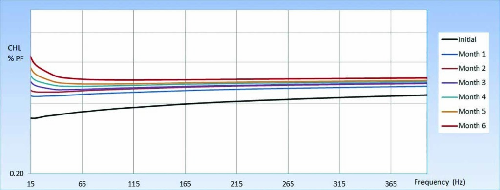
Figure 4: 97°C Responses Depicted Using a 15–400 Hertz Linear Plot
Difficulties with 60 Hertz Temperature Correction
The black trace shown in Figure 3 represents the dielectric response from a new unit. Because of negligible conductive losses, the response is dominated by the influence of static charge polarization losses. In this condition, the response trace will be remarkably linear above and below 60 hertz. This linearity results in a relationship where the applied correction is proportional to change in temperature. The slope at line frequency is positive for units in good condition; therefore, the applied correction should be upward when temperature increases.
The dielectric response for a degraded unit is depicted in the red trace in Figure 3. Because this response is driven by increasing resistive losses, the response shows significant distortion, especially at lower frequencies. This distortion results in a relationship where the applied correction is not proportional to changes in temperature. Because the slope at line frequency is negative, as temperature increases and the trace migrates to the right, the applied correction must be downward.
Conventional temperature correction tables are based on the assumption that the insulation system under test is in acceptable condition. It is therefore assumed that the slope at line frequency for this unit is positive, and that the applied correction will be reasonably proportional to temperature. Obviously, when power factor is corrected for temperature using standardized tables, the degree of correction will usually be inaccurate, and the value will be corrected in the wrong direction in some cases.
Effects of Temperature and Winding Condition
To further investigate this relationship, SCE performed an investigative study using three transformers with differing conditions. The dielectric responses for each unit were recorded as the temperature was gradually and incrementally raised from 18⁰C to 60⁰C over a period of several weeks. The first specimen was a new unit with the trough located at 10 hertz. The second unit had been removed from service with the response trough located at 55 hertz. The final unit, also removed from service, had been more heavily loaded and had a response trough located at 110 hertz.
The dielectric response of the new unit is very linear between 4–400 hertz as illustrated by the red trace in Figure 5A. As temperature is increased from 18°C, the CHL at 60 hertz remains remarkably stable past 45°C. This results in a linear temperature correction factor (TCF) from 18°C–45C as shown in Figure 6B. As the temperature rises above 45°C, the trough moves past 60 hertz and the TCF begins to trend downwards.
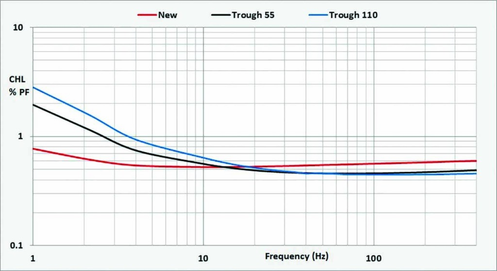
Figure 5A: NBDFR CHL — Three Specimens
As the temperature is increased for specimen 55, the CHL initially begins to decrease slightly as illustrated in the black trace in Figure 5B. As the trough moves past 60 hertz, the CHL begins to increase, rising to a greater magnitude than that shown for the new specimen. This is due to elevated watt losses from contaminants. The TCF in Figure 6B exhibits a hump from 18–30 hertz, which corresponds to the trough moving past 60 hertz.
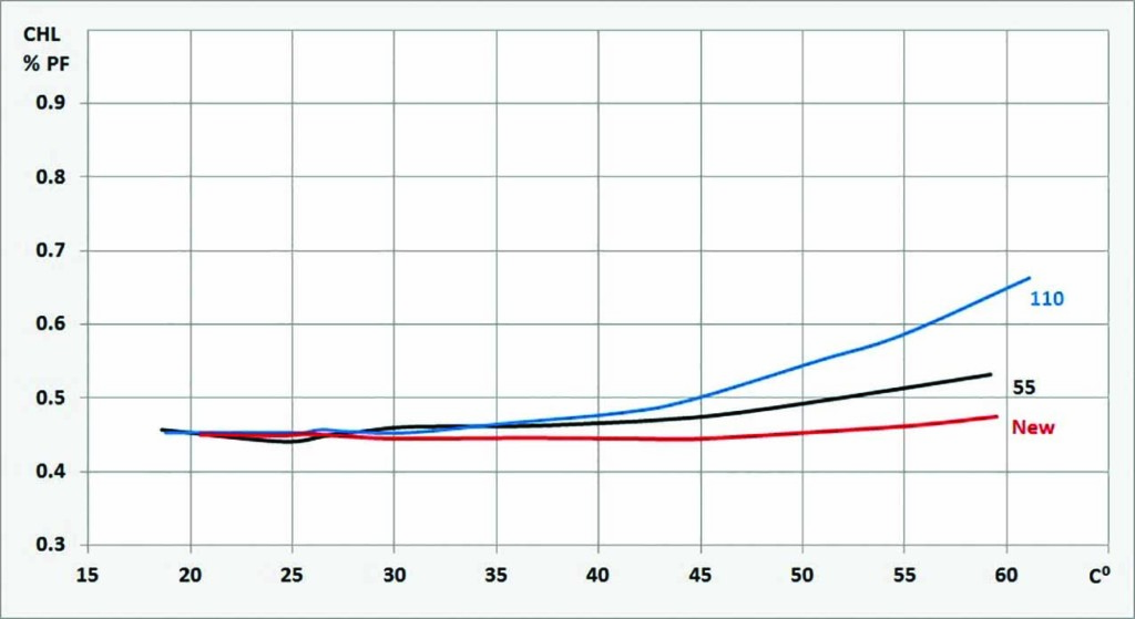
Figure 5B: CHL vs. Temperature
The CHL for specimen 110 rises immediately as temperature rises due to the fact that the trough is well past 60 hertz (Figure 5B). The magnitude of rise for CHL is much greater than that generated by specimen 55 due to even higher watt losses. This is illustrated in the divergent TCFs (Figure 6B).
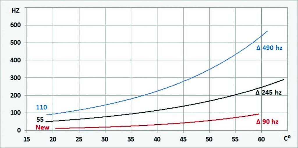
Figure 6A: Trough Position vs. Temperature
The traces in Figure 6A illustrate the changes in trough location for the three test specimens as temperature increases. The magnitude of response movement is also heavily influenced by the levels of contaminants within the oil and paper. The trough for the new specimen moves 90 hertz from 18°C to 60°C. Conversely, the trough for specimen 55 migrated 245 hertz, while the trough for specimen 110 migrated 490 hertz.
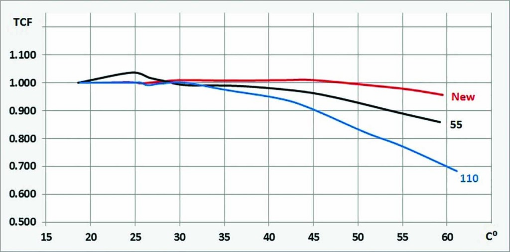
Figure 6B: TCF vs. Temperature
Influence of Winding Geometry
It has been established that conductive and polarization losses become increasingly visible at lower frequencies as capacitive current decreases. In addition to this relationship, the influence of winding geometry must be considered. With interfacial polarization (IFP), charged particles separate and move in response to the applied field, resulting in the accumulation of positive and negative charges at the interfaces of dissimilar dielectrics.
In this scenario, charged particles accumulate at the edges of the cellulose material surrounded by insulating mineral oil. This process generates measurable watt losses below 10 hertz. IFP is driven by winding geometry. The CHL interface surface area creates the mechanism by which IFP losses may be generated. The influence of IFP on higher-voltage class transformers is profound versus distribution class transformers where this influence is minimal. This relationship is demonstrated in Figure 7, which features the responses of two new units that are identical, except that one unit’s primary winding is
95 kV BIL class, while the second unit is 200 kV BIL class. In the 200 kV BIL specimen, the magnitude at 1 hertz is significantly elevated with the trough located at 40 hertz versus 4 hertz for the 95 kV BIL specimen.

Figure 7: 95 kV BIL vs. 200 kV BIL Winding Responses
Secondary Bushing Contamination
A 750 kVA transformer was subjected to condition assessment testing following removal from service. After a cursory turns-ratio test verified that the windings were intact, a narrow band DFR CHL test was performed. From 4–400 hertz, the response resembles a classic case of a transformer that has been subjected to overload conditions (Figure 8). Below 4 hertz, however, the rate of climb decreases, with the response leveling off at 2 hertz. The magnitude actually decreases slightly at 1 hertz. If the operator is astute in terms of understanding the nature of the DFR response, this scenario is particularly troubling because it is theoretically impossible unless a serious abnormal condition exists. In this case, salt fog contamination on the secondary bushings created a condition that generated parallel path watt losses, thereby distorting the response. The condition was mitigated, resulting in a normal response.
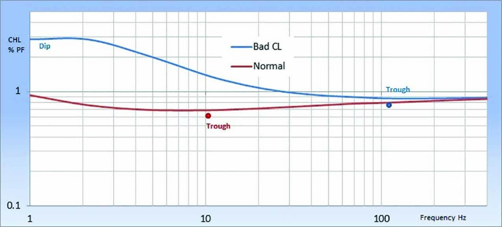
Figure 8: NBDFR CHL Measurements Before and After Cleaning of Secondary Bushings
Conclusion
The NBDFR CHL response is profoundly sensitive to changes in conductive losses. With this method, changes in condition that would be undetectable at 60 hertz can be clearly seen at lower frequencies. It should be noted, however, that to differentiate between conductive losses due to moisture versus degraded insulation, full-frequency DFR must be used.
To obtain consistently accurate assessments, a robust database must be maintained to establish optimum responses for each transformer type in the utility inventory.
When utilizing the NBDFR technique, the technician must be cognizant of the effects of temperature, especially when ambient conditions in field applications are well above or below 20°C. The technician’s most significant challenge is to discern normal versus abnormal responses. Differing geometric influences are encountered when multiple manufacturers and voltage classes are evaluated, making interpretation problematic for the novice technician. This may be especially difficult when working with distribution-class units where greater variation is seen between identical units.
References
Breazeal, R. “Narrow Band Dielectric Frequency Response and Transformer Condition Assessment,” NETA 2018.
Duplessis, J. “Electrical Field Tests for the Life Management of Transformers,” OMICRON Electronics 2013.
Breazeal, R. “Effects of Loading on Insulation Degradation as Detected in Narrow Band Dielectric Frequency Response,” Weidmann 2017.
Breazeal, R. and Chhajer, D., “Expanding the Diagnostic Impact of Power Factor Testing,” Transformers Magazine, April 2019.
 Robert Breazeal has specialized in condition assessment of power transformers at SCE for 35 years and is a leading practitioner of NBDFR in North America, testing nearly 2,000 transformers annually. Robert has authored numerous white papers and articles detailing the research and diagnostic protocols developed at SCE. Robert currently provides technical oversight for transformer repairs at the SCE Westminster Distribution Apparatus Facility and analytical support for the Distribution Apparatus Engineering and Root Cause Analysis groups.