

Since its inception in the early 20th century, testing grounded electrodes has been grounded on one technique and technology only: Fall of Potential. The test instrument made contact with the earth through long leads and driven probes, injected a current between the electrode being tested and a remote probe, and measured the voltage drop caused by earth resistance to another driven probe. Since the earth is not a discrete object, but rather the vastness of the planet, ground testing required a great deal of operator training, knowledge, involvement, and technique to obtain a reliable measurement and confirm it was correct.
Over the years, improvements accrued with three goals: Make the tests less time consuming, more accurate, and more reliable. In the late 20th century, a second technology — the clamp-on ground tester — emerged. However, the clamp-on aims only at the first of the three goals: make testing quicker and easier. It eliminates long leads and a lot of walking to move probes. However, it is somewhat less accurate, less reliable, and includes significant limitations, specifically shorts and opens — the two fundamental faults in electrical operations of all sorts. A clamp-on can’t test an isolated electrode not connected to a system (open) or to a multiply-connected electrode (short).
About the same time, the computer-based grounding multimeter was developed. This is not actually a new technology, but rather a significant enhancement of the tried-and-true Fall of Potential and its derivatives. Developed by A. P. (Sakis) Meliopoulos in association with George Cokkinides at Georgia Tech and then commercially marketed, the grounding multimeter combines standard testing techniques with computer-controlled interaction that vastly enhances data analysis. Operation is back to square one in terms of time and involvement, but built-in computer analysis adds another layer of confidence in accuracy and reliability. The original ground testers were null balance instruments that worked by balancing a series of built-in decade resistors against the load, which was the critical expanse of earth judiciously selected by the operator for probe placement. The reading was attained when the null meter balanced. Instrument technology at the time was concerned with getting an accurate measurement; it left a lot for the operator to figure out when a stable reading was not forthcoming, and a lot of trial and error was routine. Later, built-in indicators detected issues such as noise interference and insufficient probe contact and notified the operator. Additional test methods dealt with common problems like working distance and used mathematics to flag insufficient tests and give the operator the chance to try again after some correction.
The computer-based multimeter still relies on the traditional knowledge and parameters of ground testing, so the operator’s experience is not supplanted. Rather, it is supplemented by software that adds an extra layer of accuracy and confidence in the results. The multimeter works in tandem with a computer to perform ground impedance, soil resistivity, step and touch potentials, continuity, ground mat impedance, and tower ground resistance measurements — all within an operator’s basic understanding of these tests. Using leads and probes in the soil, the multimeter injects a square wave current signal and measures the voltage drop according to established ground testing principles (Figure 1). But the resulting data doesn’t end at the display. The software analyzes it for coherence and agreement and provides the operator with a confidence factor.
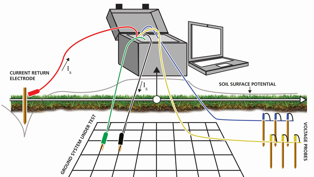
Figure 1: A computer-based test system uses standard test technology coupled with computer control and data analysis.
One significant improvement over standard earth testers is that the multimeter employs six potential parallel and stationary probes instead of the traditional single probe that must be repeatedly moved by the operator. The software analyses the soil environment around the probes and averages out the most reliable reading while storing the information for operator review. The operator is not held hostage by the software, but rather is constantly updated on the screen and afforded a high degree of flexibility in modifying the parameters. The software first collects data to calibrate the potential probe. A second phase collects ground potential data to compute the ground system impedance. The probe calibration phase eliminates any undue influence probe resistance might otherwise exert on the measurement. The data is retained internally, but is also posted on the screen. It includes the resistance, inductance, and percent error of each of the six probes (Figure 2). The operator can make a decision, adjust probes, and restart the test until satisfied.
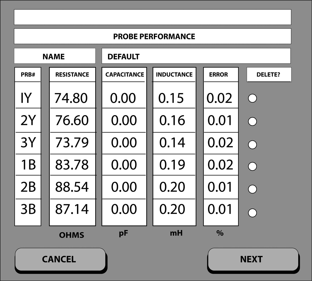
Figure 2: Test Results Display
Testing proceeds and displays another report on data quality. To calculate this report, the software considers corrupted data where harmonics or other noise sources have contributed excessively and assigns a percentage error. Rather than relying on a single noise indicator, as in less detailed testing methods, the operator has a clear picture of noise influence and can decide whether it is acceptable or not. A quality column provides endorsement: excellent, good, marginal, or unacceptable (Figure 3).
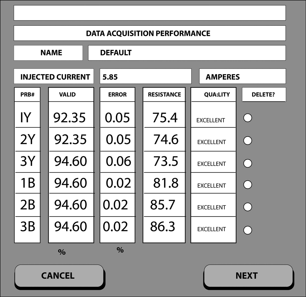
Figure 3: Data Quality Report
Unacceptable data is automatically removed from the calculation process. The operator may also remove data, and the tester offers a warning if too much is deleted. A warning is also automatically issued when probe placement is not acceptable, such as too close to another element in the system. This gives the operator an extra layer of confidence in the result. A final report calculates a probe performance index (PPI), which the operator uses to decide whether the test results are acceptable. The PPI ranges from 0 to 1, with anything below 0.5 considered good. Above 0.5, the recommendation is to reposition the probes and repeat the test (Figure 4).
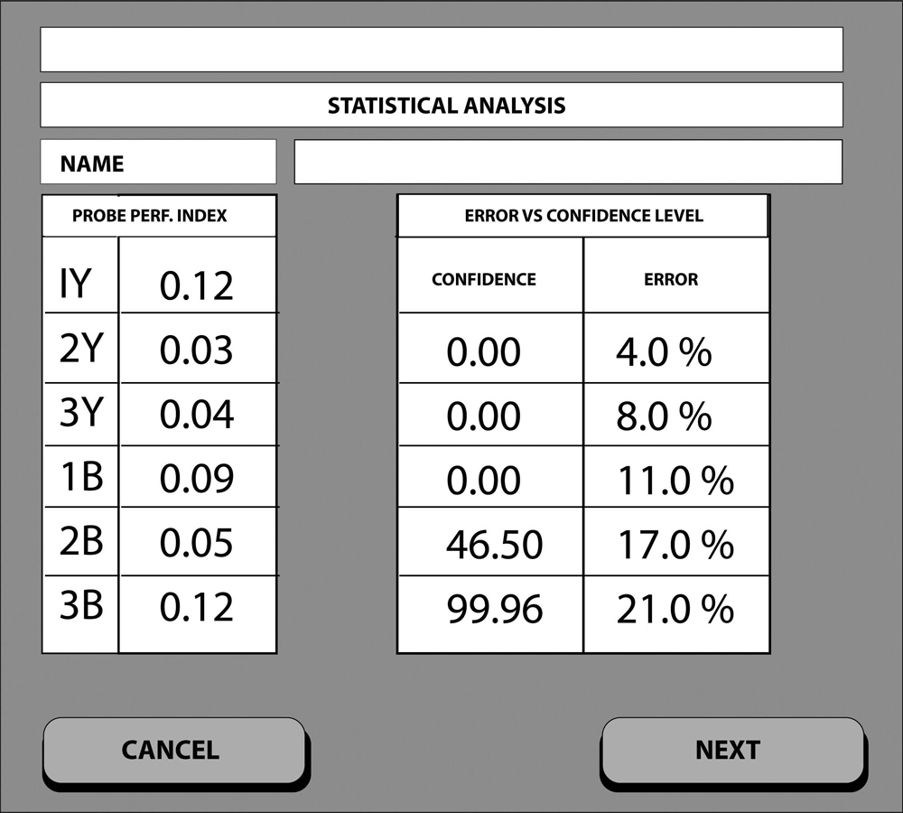
Figure 4: Probe Performance Index
How does this compare to more familiar ground testing methods with core instrumentation? Other methods sometimes result in a Fall of Potential graph that is dead flat through the middle of the range. But it is often not truly flat — the graph line wavers. Is it significant to the interpretation or just an artifact of graded landscape? And just where on the slightly wavering graph line is the actual measurement? Is it at the 62-percent point, or could that be over a water main? Typically, the resolution to this conundrum lies in the operator’s judgment. The computer-based multimeter adds a new dimension of confidence. As in traditional testing, moving the probes is the solution. But now, the software provides an objective standard, and there is less guesswork. Based on the dimensional parameters the operator enters prior to initiating the test, the software can use this ideal-case scenario to calculate results and to recognize deviations that may impinge on the accuracy of the measurements.
As with standard testing methods and equipment, soil resistivity is measured by a specific arrangement of probes. In this method, nine probes are uniformly spaced along a line on the soil surface (Figure 5). The tester collects measurements that are processed by error-correction and estimation algorithms to construct a two-layer soil model and reports the resistivities of the layers and upper layer thickness, along with an error-versus-confidence level.
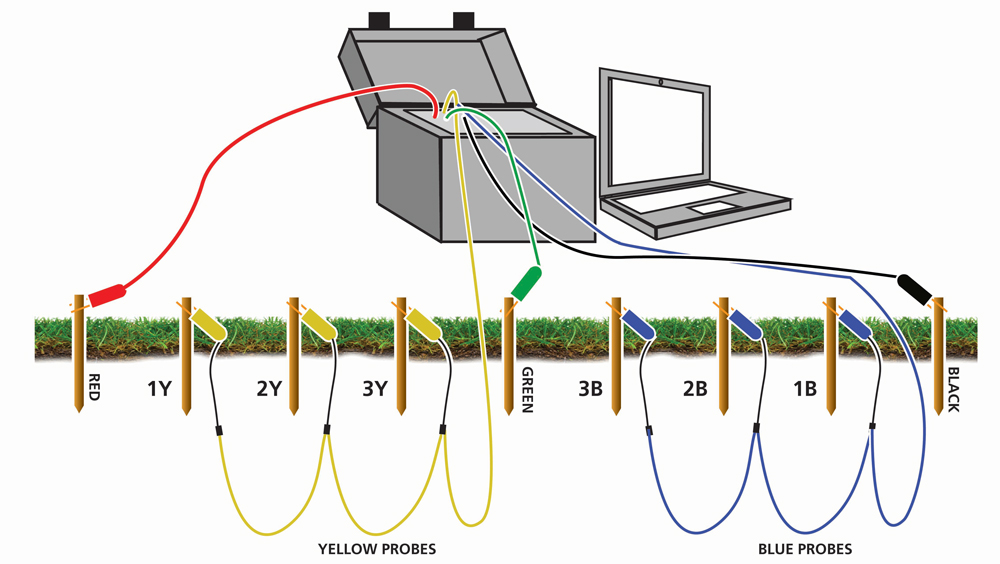
Figure 5: Soil Resistivity Setup
Transmission towers can also be tested with shield wires in place. A current is injected into the tower ground and measurements are taken to six voltage probes around the tower (Figure 6). The parallel ground resistance and the impedance looking into the shield wires are computed, and an identification algorithm determines the contribution of the shield wires and eliminates it from the total measured impedance. The algorithm separates the predominantly reactive shield impedance from the resistive ground impedance. No knowledge of shield wire parameters is necessary. The results plot tower ground impedance as a function of frequency and measure the error-versus-confidence level.
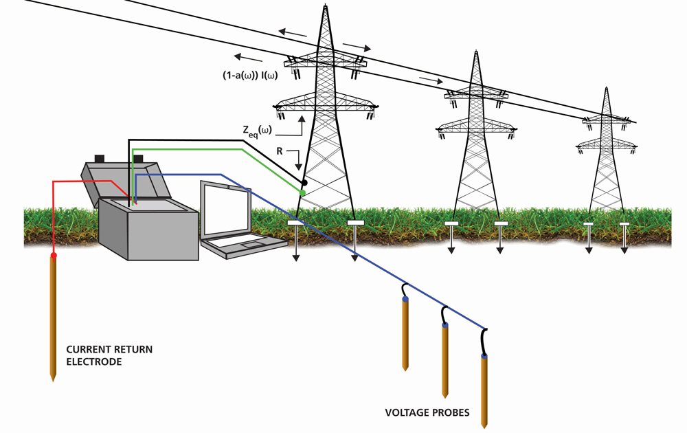
Figure 6: Tower Ground Test
Step and touch potentials, transfer voltage, and ground mat impedance are also measured. Each is defined by the probe connections and data input. Step and touch potentials require knowledge of available fault current, as do other test instruments. The computer-based multimeter also requires the operator to input the voltage, the current probe coordinates, and the size and shape of the grounding system. Transfer voltage is calculated to a user-selected point, and the coordinates are entered into the software along with the coordinates of the current return electrode, the size and location of the system, and the available fault current.
Conclusion
Using this advanced instrument and technique still relies on the tried-and-true measurement operations that were established and proven at the inception of ground testing. The operator still establishes a distinct test signal through the soil and critically places sensing probes used by the instrument to make its calculations. But the software can process an enormous number of data points to reach conclusions about accuracy and reliability that are a substantial step above human judgment when eyeballing test results. Many applications do not require this degree of specificity. But for large and complex grounding systems and where third party involvement, extensive record-keeping and auditing are important, the computer-based multimeter affords incontestable results.
References
IEEE Standard Std. 81-2012, IEEE Guide for Measuring Earth Resistivity, Ground Impedance, and Earth Surface Potentials of a Grounding System.
 Jeffrey R. Jowett is a Senior Applications Engineer for Megger in Valley Forge, Pennsylvania, serving the manufacturing lines of Biddle, Megger, and Multi-Amp for electrical test and measurement instrumentation. He holds a BS in biology and chemistry from Ursinus College. He was employed for 22 years with James G. Biddle Co., which became Biddle Instruments and is now Megger.